David R Elliott, Andrew D Thomas, Stephen R Hoon, Robin Sen
This html file is generated from source file kalahari_BSC_bacteria.Rmd which is the basis of all analyses presented in the above paper. The .Rmd file can be consulted to find the R commands used in the analyses.
## phyloseq-class experiment-level object
## otu_table()   OTU Table:         [ 2922 taxa and 48 samples ]
## sample_data() Sample Data:       [ 48 samples by 23 sample variables ]
## tax_table()   Taxonomy Table:    [ 2922 taxa by 7 taxonomic ranks ]
Chloroplast and mitochondrial sequences were removed after import (very few reads).
The full data set was used with original count data and without rarefaction, according to recommendation of the phyloseq and vegan documentation. Rarefaction was used in an earlier version of the analysis. With rarefaction to 437 sequences (excluding 2 samples) the results and statistical tests (see later) followed almost exactly the same profile, although the absolute values changed a bit.
Sequence observations were converted to percentage for each sample, to allow comparison between samples of different sequencing depth.
OTUs accounting for < 0.01% of sequences found in the study were excluded from ordinations.
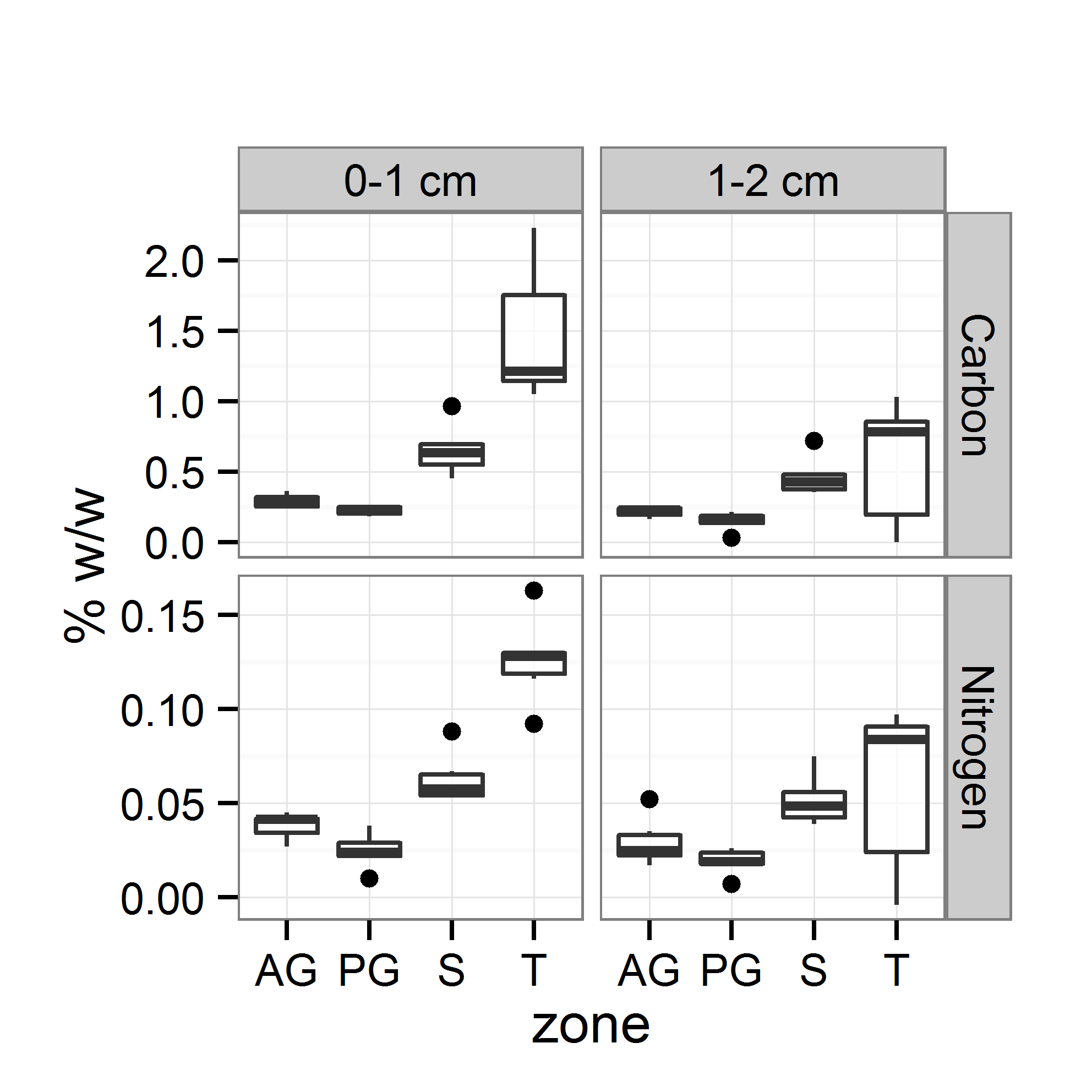
Figure 2. Total carbon and nitrogen in crust and subsoil samples at each site (n=6). Boxes represent the interquartile range (IQR), and error bars extend to the most extreme values within 1.5 * IQR of the box. Median values are shown as a line within the box and outliers are shown as black spots. Sample coding: AG=annual grass, PG=perennial grass, S=shrub, T=tree.
Figure 3. OTU richness estimation (Chao1) and diversity index (Shannon) in crust and subsoil. a. Comparison of measures at each site; b. Individual sample richness/diversity with respect to sample carbon content. Boxes represent the interquartile range (IQR), and error bars extend to the most extreme values within 1.5 * IQR of the box. Median values are shown as a line within the box and outliers are shown as black spots. Sample coding: AG=annual grass, PG=perennial grass, S=shrub, T=tree.
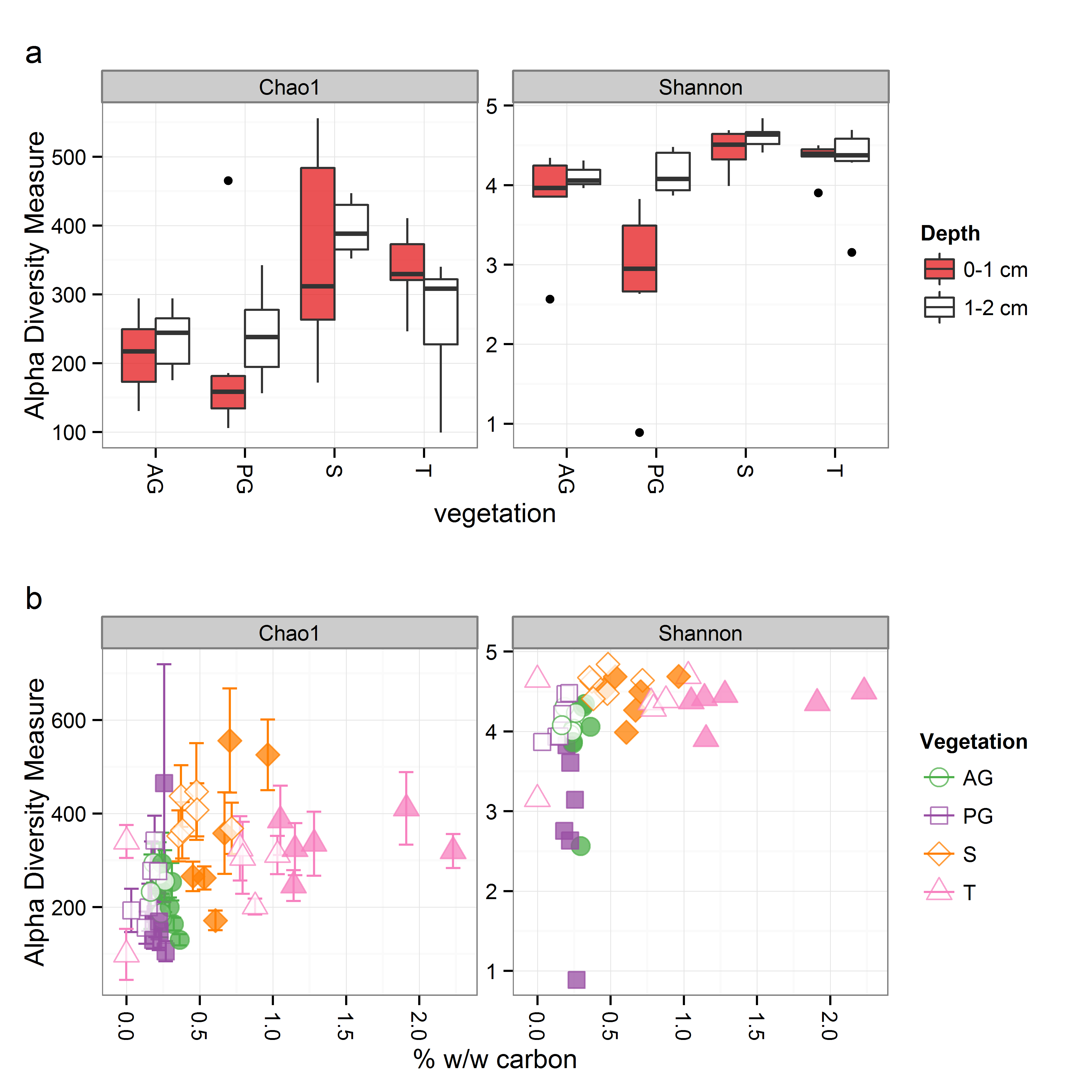
Figure 4. Phylum abundance by (a) site and (b) soil carbon content. Boxes represent the interquartile range (IQR), and error bars extend to the most extreme values within 1.5 * IQR of the box. Median values are shown as a line within the box and outliers are shown as black spots. Sample coding: AG=annual grass, PG=perennial grass, S=shrub, T=tree. Significance and direction of correlation between phylum abundance and soil carbon is indicated by + or - (determined by Spearman test). Significance codes for positive correlation: +++ < 0.001; ++ < 0.01; + <0.05. Similar plots for less abundant phyla are included in supplementary data.
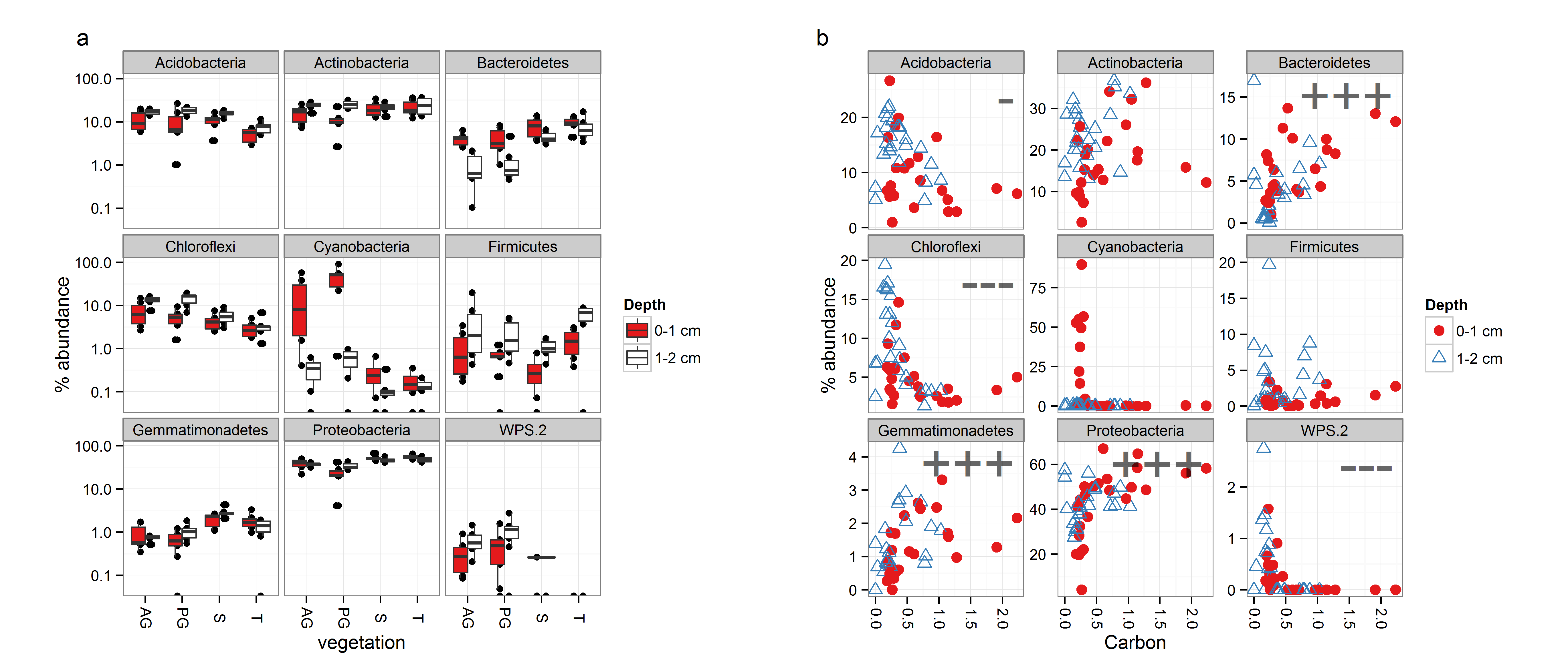
Figure 5. Correspondence analysis of the microbial community. Coloured markers indicate individual samples, and dispersion ellipses show the 95 % standard deviation confidence interval for crust/subsoil and canopy/open classifications. OTU identification numbers are shown in different colours for the 9 most abundant OTUs belonging to the followng groups: full dataset (black), phylum Cyanobacteria (green), and phylum Bacteroidetes (blue). Environmental variables with significance p < 0.05, are shown as biplotted vectors (based on permutation tests; n=1000).
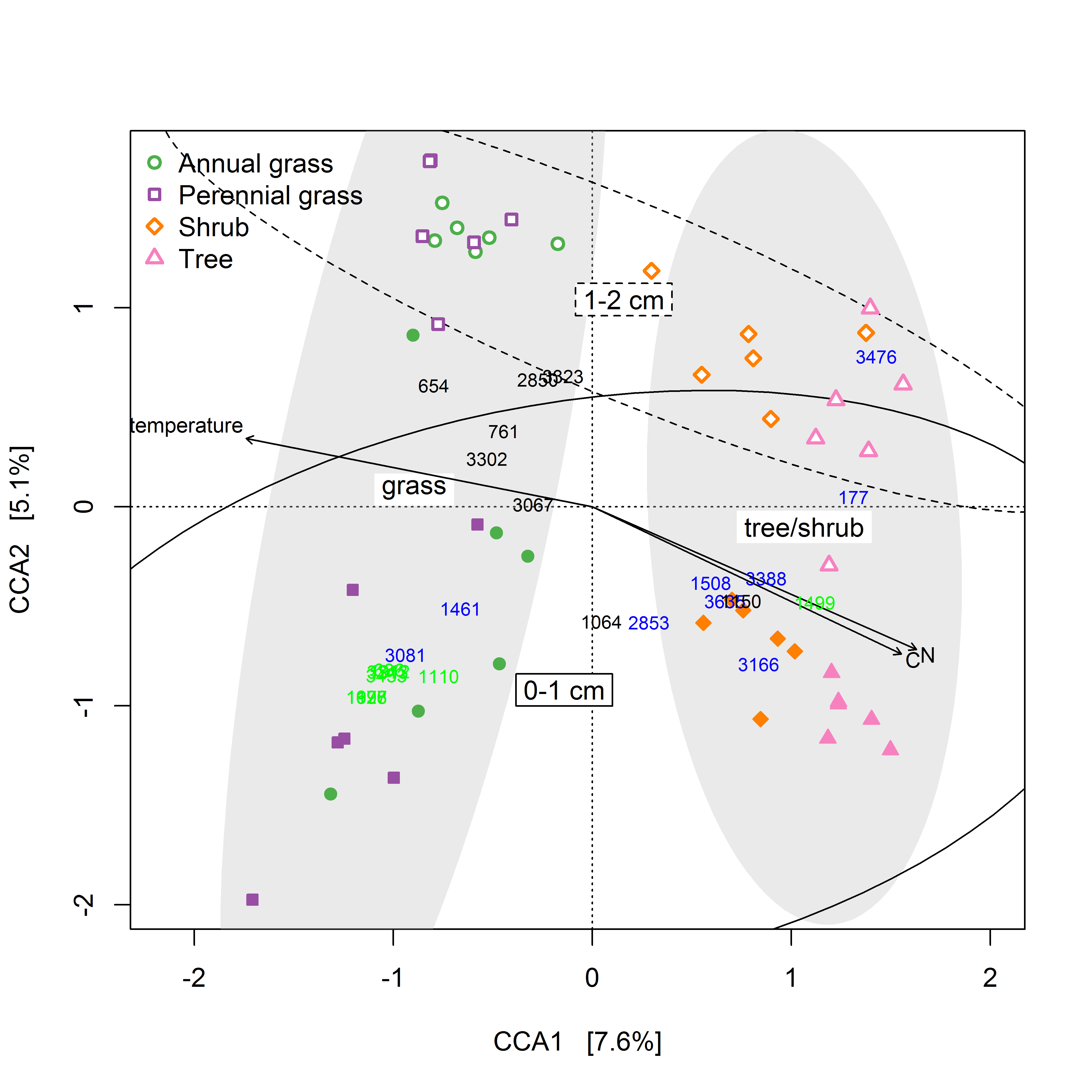
Figure 6. Relative abundance of the top 9 OTUs detected in the study, by (a) site and (b) soil carbon content. Boxes represent the interquartile range (IQR), and error bars extend to the most extreme values within 1.5 * IQR of the box. Median values are shown as a line within the box and outliers are shown as black spots. Significance and direction of correlation between OTU abundance and soil carbon is indicated by + or - (determined by Spearman test). Significance codes for positive correlation: +++ < 0.001; ++ < 0.01; + <0.05. Sample coding: AG=annual grass, PG=perennial grass, S=shrub, T=tree.
Figure 7. Relative abundance of the top 9 OTUs from the phyla (a) Bacteroidetes; (b) Cyanobacteria. Boxes represent the interquartile range (IQR), and error bars extend to the most extreme values within 1.5 * IQR of the box. Median values are shown as a line within the box and outliers are shown as black spots. Sample coding: AG=annual grass, PG=perennial grass, S=shrub, T=tree. Similar plots for other phyla are included in supplementary data.
Table 1. Significance of factors depth, vegetation, and month on phylum abundance, as determined by Kruskal Wallis test. Significant effects were further tested by post-hoc analysis which is provided as supplementary material. Significance codes: *** < 0.001; ** < 0.01; * <0.05.
| Phylum | type_sig | zone_sig | month_sig | |
|---|---|---|---|---|
| Acidobacteria | Acidobacteria | ** | ** | |
| Proteobacteria | Proteobacteria | *** | ||
| Bacteroidetes | Bacteroidetes | ** | *** | |
| Firmicutes | Firmicutes | ** | . | |
| Gemmatimonadetes | Gemmatimonadetes | *** | ||
| Cyanobacteria | Cyanobacteria | ** | ** | |
| WPS.2 | WPS-2 | *** | ||
| Chloroflexi | Chloroflexi | * | *** | |
| Actinobacteria | Actinobacteria | ** |
Table 2. Taxonomic classification of the most abundant 9 OTUs found in the study. Significance of depth, vegetation and month on OTU abundance is indicated by *** p < 0.001; ** p < 0.01; * p < 0.05, as determined by Kruskal Wallis test. Significant effects were further tested by post-hoc analyses which are provided as supplementary material.
| Phylum | Class | Order | Family | Genus | type_sig | zone_sig | month_sig | |
|---|---|---|---|---|---|---|---|---|
| 654 | Proteobacteria | Alphaproteobacteria | Rhodospirillales | Acetobacteraceae | *** | |||
| 761 | Acidobacteria | Solibacteres | Solibacterales | Solibacteraceae | Candidatus Solibacter | . | *** | |
| 1064 | Proteobacteria | Alphaproteobacteria | Rhizobiales | Methylobacteriaceae | Methylobacterium | *** | ||
| 1150 | Proteobacteria | Alphaproteobacteria | Rhizobiales | Bradyrhizobiaceae | Balneimonas | * | *** | |
| 1912 | Cyanobacteria | Oscillatoriophycideae | Oscillatoriales | Phormidiaceae | Phormidium | *** | * | |
| 2850 | Proteobacteria | Alphaproteobacteria | Rhodospirillales | Rhodospirillaceae | *** | ** | ||
| 3067 | Proteobacteria | Alphaproteobacteria | Rhodospirillales | Acetobacteraceae | * | |||
| 3302 | Actinobacteria | Actinobacteria | Actinomycetales | Kineosporiaceae | *** | |||
| 3323 | Actinobacteria | Actinobacteria | Actinomycetales | Pseudonocardiaceae | *** |
Table 3. Taxonomic classification of the most abundant 9 Bacteroidetes and Cyanobacteria OTUs found in the study. Significance of depth, vegetation and month on OTU abundance is indicated by *** p < 0.001; ** p < 0.01; * p < 0.05, as determined by Kruskal Wallis test. Significant effects were further tested by post-hoc analyses which are provided as supplementary material.
| Phylum | Class | Order | Family | Genus | type_sig | zone_sig | month_sig | |
|---|---|---|---|---|---|---|---|---|
| 177 | Bacteroidetes | Sphingobacteriia | Sphingobacteriales | Chitinophagaceae | ** | |||
| 1461 | Bacteroidetes | Sphingobacteriia | Sphingobacteriales | Chitinophagaceae | Flavisolibacter | . | ||
| 1508 | Bacteroidetes | Sphingobacteriia | Sphingobacteriales | Chitinophagaceae | Flavisolibacter | |||
| 2853 | Bacteroidetes | Sphingobacteriia | Sphingobacteriales | Chitinophagaceae | ||||
| 3081 | Bacteroidetes | Sphingobacteriia | Sphingobacteriales | Flexibacteraceae | ** | * | ||
| 3166 | Bacteroidetes | Sphingobacteriia | Sphingobacteriales | Chitinophagaceae | Segetibacter | |||
| 3388 | Bacteroidetes | Sphingobacteriia | Sphingobacteriales | Chitinophagaceae | Segetibacter | |||
| 3476 | Bacteroidetes | Sphingobacteriia | Sphingobacteriales | Chitinophagaceae | ||||
| 3635 | Bacteroidetes | Sphingobacteriia | Sphingobacteriales | Chitinophagaceae |
| Phylum | Class | Order | Family | Genus | type_sig | zone_sig | month_sig | |
|---|---|---|---|---|---|---|---|---|
| 686 | Cyanobacteria | Oscillatoriophycideae | * | * | ||||
| 1110 | Cyanobacteria | Oscillatoriophycideae | * | |||||
| 1198 | Cyanobacteria | Oscillatoriophycideae | ||||||
| 1499 | Cyanobacteria | 4C0d-2 | MLE1-12 | |||||
| 1626 | Cyanobacteria | Oscillatoriophycideae | ||||||
| 1912 | Cyanobacteria | Oscillatoriophycideae | Oscillatoriales | Phormidiaceae | Phormidium | ** | * | |
| 1977 | Cyanobacteria | Oscillatoriophycideae | . | |||||
| 3313 | Cyanobacteria | Oscillatoriophycideae | . | * | ||||
| 3453 | Cyanobacteria | Oscillatoriophycideae | Oscillatoriales | Phormidiaceae |
This section includes supplementary plots, and statistical tests supporting statements made in the manuscript. Additional plots and tests can be found by following links in this document or exploring the results folders.
This analysis was performed using adonis() function of the vegan package, which is described as follows:
Analysis of variance using distance matrices - for partitioning distance matrices among sources of variation and fitting linear models (e.g., factors, polynomial regression) to distance matrices; uses a permutation test with pseudo-F ratios.
## The same test was run at each taxonomic rank.
##
##
## __ Phylum __
## Run 0 stress 0.0963
## Run 1 stress 0.09618
## ... New best solution
## ... procrustes: rmse 0.003268  max resid 0.01563
## Run 2 stress 0.09618
## ... procrustes: rmse 0.001116  max resid 0.006303
## *** Solution reached
##
##
## Call:
## adonis(formula = dist ~ zone * type + month, data = as(sample_data(expt.ord.taxrank),      "data.frame"))
##
## Terms added sequentially (first to last)
##
##           Df SumsOfSqs MeanSqs F.Model    R2 Pr(>F)
## zone       3      0.99   0.329    4.24 0.200  0.001 ***
## type       1      0.37   0.374    4.82 0.076  0.001 ***
## month      1      0.06   0.063    0.81 0.013  0.520
## zone:type  3      0.50   0.165    2.13 0.100  0.013 *
## Residuals 39      3.03   0.078         0.612
## Total     47      4.95                 1.000
## ---
## Signif. codes:  0 '***' 0.001 '**' 0.01 '*' 0.05 '.' 0.1 ' ' 1
##
##
## __ Class __
## Run 0 stress 0.1129
## Run 1 stress 0.1129
## ... procrustes: rmse 0.0004617  max resid 0.002663
## *** Solution reached
##
##
## Call:
## adonis(formula = dist ~ zone * type + month, data = as(sample_data(expt.ord.taxrank),      "data.frame"))
##
## Terms added sequentially (first to last)
##
##           Df SumsOfSqs MeanSqs F.Model    R2 Pr(>F)
## zone       3      1.30   0.432    5.01 0.225  0.001 ***
## type       1      0.45   0.446    5.17 0.078  0.001 ***
## month      1      0.11   0.113    1.31 0.020  0.238
## zone:type  3      0.53   0.177    2.05 0.092  0.008 **
## Residuals 39      3.36   0.086         0.585
## Total     47      5.75                 1.000
## ---
## Signif. codes:  0 '***' 0.001 '**' 0.01 '*' 0.05 '.' 0.1 ' ' 1
##
##
## __ Order __
## Run 0 stress 0.1443
## Run 1 stress 0.139
## ... New best solution
## ... procrustes: rmse 0.09186  max resid 0.2292
## Run 2 stress 0.1443
## Run 3 stress 0.1598
## Run 4 stress 0.1609
## Run 5 stress 0.1388
## ... New best solution
## ... procrustes: rmse 0.01621  max resid 0.08933
## Run 6 stress 0.1845
## Run 7 stress 0.1443
## Run 8 stress 0.1705
## Run 9 stress 0.1629
## Run 10 stress 0.139
## ... procrustes: rmse 0.01616  max resid 0.08978
## Run 11 stress 0.1676
## Run 12 stress 0.1609
## Run 13 stress 0.1388
## ... New best solution
## ... procrustes: rmse 0.0007276  max resid 0.002895
## *** Solution reached
##
##
## Call:
## adonis(formula = dist ~ zone * type + month, data = as(sample_data(expt.ord.taxrank),      "data.frame"))
##
## Terms added sequentially (first to last)
##
##           Df SumsOfSqs MeanSqs F.Model    R2 Pr(>F)
## zone       3      1.52   0.508    5.53 0.243  0.001 ***
## type       1      0.50   0.501    5.46 0.080  0.001 ***
## month      1      0.16   0.161    1.75 0.026  0.110
## zone:type  3      0.51   0.169    1.84 0.081  0.021 *
## Residuals 39      3.58   0.092         0.571
## Total     47      6.28                 1.000
## ---
## Signif. codes:  0 '***' 0.001 '**' 0.01 '*' 0.05 '.' 0.1 ' ' 1
##
##
## __ Family __
## Run 0 stress 0.1508
## Run 1 stress 0.1512
## ... procrustes: rmse 0.01017  max resid 0.05234
## Run 2 stress 0.1578
## Run 3 stress 0.1512
## ... procrustes: rmse 0.009412  max resid 0.05358
## Run 4 stress 0.1601
## Run 5 stress 0.1614
## Run 6 stress 0.1512
## ... procrustes: rmse 0.01069  max resid 0.05198
## Run 7 stress 0.1807
## Run 8 stress 0.1603
## Run 9 stress 0.1601
## Run 10 stress 0.1508
## ... New best solution
## ... procrustes: rmse 0.0003335  max resid 0.00194
## *** Solution reached
##
##
## Call:
## adonis(formula = dist ~ zone * type + month, data = as(sample_data(expt.ord.taxrank),      "data.frame"))
##
## Terms added sequentially (first to last)
##
##           Df SumsOfSqs MeanSqs F.Model    R2 Pr(>F)
## zone       3      2.13   0.710    6.13 0.255  0.001 ***
## type       1      0.80   0.804    6.95 0.096  0.001 ***
## month      1      0.25   0.253    2.19 0.030  0.037 *
## zone:type  3      0.64   0.212    1.83 0.076  0.015 *
## Residuals 39      4.51   0.116         0.542
## Total     47      8.34                 1.000
## ---
## Signif. codes:  0 '***' 0.001 '**' 0.01 '*' 0.05 '.' 0.1 ' ' 1
##
##
## __ Genus __
## Run 0 stress 0.1644
## Run 1 stress 0.1408
## ... New best solution
## ... procrustes: rmse 0.08226  max resid 0.513
## Run 2 stress 0.1408
## ... New best solution
## ... procrustes: rmse 0.00179  max resid 0.009651
## *** Solution reached
##
##
## Call:
## adonis(formula = dist ~ zone * type + month, data = as(sample_data(expt.ord.taxrank),      "data.frame"))
##
## Terms added sequentially (first to last)
##
##           Df SumsOfSqs MeanSqs F.Model    R2 Pr(>F)
## zone       3      2.51   0.838    5.56 0.233  0.001 ***
## type       1      1.43   1.427    9.46 0.132  0.001 ***
## month      1      0.26   0.261    1.73 0.024  0.102
## zone:type  3      0.72   0.239    1.58 0.066  0.031 *
## Residuals 39      5.88   0.151         0.545
## Total     47     10.80                 1.000
## ---
## Signif. codes:  0 '***' 0.001 '**' 0.01 '*' 0.05 '.' 0.1 ' ' 1
##
##
## __ Species __
## Run 0 stress 0.1533
## Run 1 stress 0.1545
## Run 2 stress 0.1666
## Run 3 stress 0.1533
## ... New best solution
## ... procrustes: rmse 0.0001408  max resid 0.0008795
## *** Solution reached
##
##
## Call:
## adonis(formula = dist ~ zone * type + month, data = as(sample_data(expt.ord.taxrank),      "data.frame"))
##
## Terms added sequentially (first to last)
##
##           Df SumsOfSqs MeanSqs F.Model    R2 Pr(>F)
## zone       3      3.48   1.158    4.88 0.227  0.001 ***
## type       1      1.17   1.172    4.94 0.076  0.001 ***
## month      1      0.34   0.342    1.44 0.022  0.096 .
## zone:type  3      1.08   0.360    1.52 0.070  0.014 *
## Residuals 39      9.26   0.237         0.604
## Total     47     15.33                 1.000
## ---
## Signif. codes:  0 '***' 0.001 '**' 0.01 '*' 0.05 '.' 0.1 ' ' 1
Phylum results:
Phylum: OTU taxonomy and statistical results
Directory containing stat tables for each test
Phylum [top 9] zone plot
Phylum [top 9] carbon plot
Phylum [top 9] tree
Abundant OTUs results:
All: OTU taxonomy and statistical results
Directory containing stat tables for each test
All [top 9] zone plot
All [top 9] carbon plot
All [top 9] tree
Bacteroidetes results:
Bacteroidetes: OTU taxonomy and statistical results
Directory containing stat tables for each test
Bacteroidetes [top 9] zone plot
Bacteroidetes [top 9] carbon plot
Bacteroidetes [top 9] tree
Cyanobacteria results:
Cyanobacteria: OTU taxonomy and statistical results
Directory containing stat tables for each test
Cyanobacteria [top 9] zone plot
Cyanobacteria [top 9] carbon plot
Cyanobacteria [top 9] tree
##              zone    type   mean      sd
## 1    Annual_grass   crust 0.2950 0.04783
## 2    Annual_grass subsoil 0.2188 0.03728
## 3 Perennial_grass   crust 0.2250 0.03259
## 4 Perennial_grass subsoil 0.1480 0.06434
## 5           Shrub   crust 0.6547 0.17715
## 6           Shrub subsoil 0.4638 0.13543
## 7            Tree   crust 1.4600 0.48875
## 8            Tree subsoil 0.5785 0.45825
##      type   mean     sd
## 1   crust 0.6587 0.5573
## 2 subsoil 0.3523 0.2880
## Analysis of Variance Table
##
## Response: map.df$Carbon
##                      Df Sum Sq Mean Sq F value  Pr(>F)
## factor(map.df$zone)   3   5.16   1.722   19.56 4.3e-08 ***
## factor(map.df$type)   1   1.13   1.126   12.80 0.00089 ***
## factor(map.df$month)  1   0.19   0.190    2.16 0.14906
## Residuals            42   3.70   0.088
## ---
## Signif. codes:  0 '***' 0.001 '**' 0.01 '*' 0.05 '.' 0.1 ' ' 1
##   Tukey multiple comparisons of means
##     95% family-wise confidence level
##     factor levels have been ordered
##
## Fit: aov(formula = map.df$Carbon ~ factor(map.df$zone) + factor(map.df$type) + factor(map.df$month))
##
## $`factor(map.df$zone)`
##                                 diff      lwr    upr  p adj
## Annual_grass-Perennial_grass 0.07042 -0.25355 0.3944 0.9371
## Shrub-Perennial_grass        0.37275  0.04878 0.6967 0.0185
## Tree-Perennial_grass         0.83275  0.50878 1.1567 0.0000
## Shrub-Annual_grass           0.30233 -0.02164 0.6263 0.0751
## Tree-Annual_grass            0.76233  0.43836 1.0863 0.0000
## Tree-Shrub                   0.46000  0.13603 0.7840 0.0025
##
## $`factor(map.df$type)`
##                 diff    lwr    upr p adj
## crust-subsoil 0.3064 0.1335 0.4792 9e-04
##
## $`factor(map.df$month)`
##           diff      lwr    upr  p adj
## Nov-Mar 0.1259 -0.04695 0.2987 0.1491
##              zone    type   mean    sd
## 1    Annual_grass   crust  7.968 2.110
## 2    Annual_grass subsoil  8.124 1.973
## 3 Perennial_grass   crust 10.403 4.356
## 4 Perennial_grass subsoil  7.581 2.216
## 5           Shrub   crust 10.320 1.147
## 6           Shrub subsoil  8.981 1.056
## 7            Tree   crust 11.452 2.375
## 8            Tree subsoil  6.546 5.041
##      type   mean    sd
## 1   crust 10.036 2.881
## 2 subsoil  7.808 2.914
## Analysis of Variance Table
##
## Response: map.df$CN
##                      Df Sum Sq Mean Sq F value  Pr(>F)
## factor(map.df$zone)   3   15.7     5.2    0.78 0.50985
## factor(map.df$type)   1   59.6    59.6    8.91 0.00471 **
## factor(map.df$month)  1   89.9    89.9   13.45 0.00068 ***
## Residuals            42  280.7     6.7
## ---
## Signif. codes:  0 '***' 0.001 '**' 0.01 '*' 0.05 '.' 0.1 ' ' 1
##   Tukey multiple comparisons of means
##     95% family-wise confidence level
##     factor levels have been ordered
##
## Fit: aov(formula = map.df$CN ~ factor(map.df$zone) + factor(map.df$type) + factor(map.df$month))
##
## $`factor(map.df$zone)`
##                                  diff    lwr   upr  p adj
## Perennial_grass-Annual_grass 0.945948 -1.877 3.769 0.8068
## Tree-Annual_grass            0.952897 -1.870 3.776 0.8033
## Shrub-Annual_grass           1.604547 -1.218 4.428 0.4347
## Tree-Perennial_grass         0.006949 -2.816 2.830 1.0000
## Shrub-Perennial_grass        0.658599 -2.164 3.482 0.9238
## Shrub-Tree                   0.651650 -2.171 3.475 0.9259
##
## $`factor(map.df$type)`
##                diff    lwr   upr  p adj
## crust-subsoil 2.228 0.7219 3.734 0.0047
##
## $`factor(map.df$month)`
##          diff   lwr   upr p adj
## Nov-Mar 2.737 1.231 4.243 7e-04
##
## Call:
## lm(formula = map.df$Nitrogen ~ map.df$Carbon)
##
## Residuals:
##       Min        1Q    Median        3Q       Max
## -0.029632 -0.007291  0.000414  0.005297  0.027902
##
## Coefficients:
##               Estimate Std. Error t value Pr(>|t|)
## (Intercept)    0.01253    0.00240    5.23  4.1e-06 ***
## map.df$Carbon  0.07702    0.00351   21.97  < 2e-16 ***
## ---
## Signif. codes:  0 '***' 0.001 '**' 0.01 '*' 0.05 '.' 0.1 ' ' 1
##
## Residual standard error: 0.0112 on 46 degrees of freedom
## Multiple R-squared:  0.913,  Adjusted R-squared:  0.911
## F-statistic:  483 on 1 and 46 DF,  p-value: <2e-16
## pdf
##   2
Check significance of correlation between richness/diversity and carbon (Spearman):
## Chao1
##  Spearman's rank correlation rho
##
## data:  carbon_richness$value and carbon_richness$Carbon
## S = 9258, p-value = 0.0003211
## alternative hypothesis: true rho is not equal to 0
## sample estimates:
##    rho
## 0.4975
##
## Shannon
##  Spearman's rank correlation rho
##
## data:  carbon_richness$value and carbon_richness$Carbon
## S = 9256, p-value = 0.00032
## alternative hypothesis: true rho is not equal to 0
## sample estimates:
##    rho
## 0.4976
Check effect of depth and vegetation zone on richness/diversity (Kruskal-Wallis):
##
##  Kruskal-Wallis rank sum test
##
## data:  rich.plus$Shannon by rich.plus$type
## Kruskal-Wallis chi-squared = 2.929, df = 1, p-value = 0.087
##
##  Kruskal-Wallis rank sum test
##
## data:  rich.plus$Shannon by rich.plus$zone_code
## Kruskal-Wallis chi-squared = 22.91, df = 3, p-value = 4.222e-05
##
##  Kruskal-Wallis rank sum test
##
## data:  rich.plus$Chao1 by rich.plus$type
## Kruskal-Wallis chi-squared = 0.5208, df = 1, p-value = 0.4705
##
##  Kruskal-Wallis rank sum test
##
## data:  rich.plus$Chao1 by rich.plus$zone_code
## Kruskal-Wallis chi-squared = 17.08, df = 3, p-value = 0.0006791
## Post-hoc test - Shannon diversity
## Multiple comparison test after Kruskal-Wallis
## p.value: 0.05
## Comparisons
##       obs.dif critical.dif difference
## AG-PG   4.417        15.08      FALSE
## AG-S   20.000        15.08       TRUE
## AG-T   12.083        15.08      FALSE
## PG-S   24.417        15.08       TRUE
## PG-T   16.500        15.08       TRUE
## S-T     7.917        15.08      FALSE
## Post-hoc test - Chao1 richness
## Multiple comparison test after Kruskal-Wallis
## p.value: 0.05
## Comparisons
##       obs.dif critical.dif difference
## AG-PG  0.6667        15.08      FALSE
## AG-S  19.2500        15.08       TRUE
## AG-T  11.7500        15.08      FALSE
## PG-S  19.9167        15.08       TRUE
## PG-T  12.4167        15.08      FALSE
## S-T    7.5000        15.08      FALSE
Constrained and Unconstrained comparison, and scree plots. The constrained ordination shown here is exactly the same as the one used for the main figure above.
Constrained and unconstrained ordinations with scree plots.
Part of Online resource 4. Relative abundance of Proteobacterial classes, by (a) site and (b) soil carbon content. Boxes represent the interquartile range (IQR), and error bars extend to the most extreme values within 1.5 * IQR of the box. Median values are shown as a line within the box and outliers are shown as black spots. Significance and direction of correlation between OTU abundance and soil carbon is indicated by + or - (determined by Spearman test). Significance codes for positive correlation: +++ < 0.001; ++ < 0.01; + <0.05. Sample coding: AG=annual grass, PG=perennial grass, S=shrub, T=tree.
Top 16 phyla


Each Phylum in turn: See plots in folder figures_extra and results in statistics
print(calcs_for_manuscript)
## $`total phyla`
## [1] 28
##
## $`top 9 phyla sum`
## [1] 99.08
##
## $`top 16 phyla sum`
## [1] 99.78
##
## $`total actinobacteria`
## [1] 20.78
##
## $`total proteobacteria`
## [1] 42.02
##
## $`top 9 OTUs sum`
## [1] 26.75
##
## $`total bacteroidetes`
## [1] 5.092
##
## $`total cyanobacteria`
## [1] 8.14
##
## $`Chloroflexi n OTUs`
## [1] 408
##
## $`Chloroflexi top 9`
## [1] 2.65
##
## $`Proteobacteria n OTUs`
## [1] 935
##
## $`Proteobacteria top 9`
## [1] 17.87
##
## $`Bacteroidetes n OTUs`
## [1] 297
##
## $`Bacteroidetes top 9`
## [1] 1.786
##
## $`Elusimicrobia n OTUs`
## [1] 28
##
## $`Elusimicrobia top 9`
## [1] 0.07648
##
## $`Acidobacteria n OTUs`
## [1] 195
##
## $`Acidobacteria top 9`
## [1] 7.012
##
## $`Firmicutes n OTUs`
## [1] 67
##
## $`Firmicutes top 9`
## [1] 1.946
##
## $`Actinobacteria n OTUs`
## [1] 407
##
## $`Actinobacteria top 9`
## [1] 9.614
##
## $`TM7 n OTUs`
## [1] 28
##
## $`TM7 top 9`
## [1] 0.05468
##
## $`Armatimonadetes n OTUs`
## [1] 14
##
## $`Armatimonadetes top 9`
## [1] 0.0797
##
## $`Gemmatimonadetes n OTUs`
## [1] 176
##
## $`Gemmatimonadetes top 9`
## [1] 0.3543
##
## $`Fibrobacteres n OTUs`
## [1] 1
##
## $`Fibrobacteres top 9`
## [1] 0.002349
##
## $`Nitrospirae n OTUs`
## [1] 9
##
## $`Nitrospirae top 9`
## [1] 0.1198
##
## $`OP11 n OTUs`
## [1] 1
##
## $`OP11 top 9`
## [1] 0.00298
##
## $`Planctomycetes n OTUs`
## [1] 18
##
## $`Planctomycetes top 9`
## [1] 0.03546
##
## $`Tenericutes n OTUs`
## [1] 1
##
## $`Tenericutes top 9`
## [1] 0.001701
##
## $`OD1 n OTUs`
## [1] 16
##
## $`OD1 top 9`
## [1] 0.03273
##
## $`AD3 n OTUs`
## [1] 4
##
## $`AD3 top 9`
## [1] 0.07563
##
## $`Cyanobacteria n OTUs`
## [1] 38
##
## $`Cyanobacteria top 9`
## [1] 8.012
##
## $`TM6 n OTUs`
## [1] 8
##
## $`TM6 top 9`
## [1] 0.03761
##
## $`Thermi n OTUs`
## [1] 13
##
## $`Thermi top 9`
## [1] 0.05206
##
## $`Chlorobi n OTUs`
## [1] 12
##
## $`Chlorobi top 9`
## [1] 0.08106
##
## $`WYO n OTUs`
## [1] 3
##
## $`WYO top 9`
## [1] 0.008694
##
## $`WS2 n OTUs`
## [1] 1
##
## $`WS2 top 9`
## [1] 0.001432
##
## $`Verrucomicrobia n OTUs`
## [1] 16
##
## $`Verrucomicrobia top 9`
## [1] 0.09866
##
## $`Fusobacteria n OTUs`
## [1] 1
##
## $`Fusobacteria top 9`
## [1] 0.002634
##
## $`OP9 n OTUs`
## [1] 2
##
## $`OP9 top 9`
## [1] 0.004157
##
## $`WPS-2 n OTUs`
## [1] 5
##
## $`WPS-2 top 9`
## [1] 0.3315
##
## $`BRC1 n OTUs`
## [1] 1
##
## $`BRC1 top 9`
## [1] 0.001701
##
## $`total for top 9 of each phylum`
## [1] 50.34
print(sessionInfo(), locale = FALSE)
## R version 3.1.0 (2014-04-10)
## Platform: x86_64-w64-mingw32/x64 (64-bit)
##
## attached base packages:
## [1] grid      stats     graphics  grDevices utils     datasets  methods   base
##
## other attached packages:
##  [1] pgirmess_1.5.8     vegan_2.0-10       lattice_0.20-29    permute_0.8-3      xtable_1.7-3       RColorBrewer_1.0-5 reshape_0.8.4      plyr_1.8.1
##  [9] scales_0.2.3       ggplot2_0.9.3.1    phyloseq_1.7.24    knitr_1.5
##
## loaded via a namespace (and not attached):
##  [1] ade4_1.6-2              annotate_1.40.0         AnnotationDbi_1.24.0    ape_3.1-1               Biobase_2.22.0          BiocGenerics_0.8.0
##  [7] biom_0.3.12             Biostrings_2.30.1       boot_1.3-11             cluster_1.15.2          coda_0.16-1             codetools_0.2-8
## [13] colorspace_1.2-4        data.table_1.9.2        DBI_0.2-7               deldir_0.1-5            DESeq2_1.2.10           dichromat_2.0-0
## [19] digest_0.6.4            evaluate_0.5.3          foreach_1.4.2           formatR_0.10            genefilter_1.44.0       GenomicRanges_1.14.4
## [25] gtable_0.1.2            igraph_0.7.0            IRanges_1.20.6          iterators_1.0.7         labeling_0.2            LearnBayes_2.12
## [31] locfit_1.5-9.1          MASS_7.3-31             Matrix_1.1-3            multtest_2.18.0         munsell_0.4.2           nlme_3.1-117
## [37] parallel_3.1.0          proto_0.3-10            Rcpp_0.11.1             RcppArmadillo_0.4.200.0 reshape2_1.2.2          rgdal_0.8-16
## [43] RJSONIO_1.0-3           RSQLite_0.11.4          sp_1.0-15               spdep_0.5-71            splancs_2.01-34         splines_3.1.0
## [49] stats4_3.1.0            stringr_0.6.2           survival_2.37-7         tools_3.1.0             XML_3.98-1.1            XVector_0.2.0
![Phylum [top 9] zone plot](figures_extra/Phylum_zone.png)
![Phylum [top 9] carbon plot](figures_extra/Phylum_carbon.png)
![Phylum [top 9] tree](figures_extra/Phylum_tree.png)
![All [top 9] zone plot](figures_extra/All_zone.png)
![All [top 9] carbon plot](figures_extra/All_carbon.png)
![All [top 9] tree](figures_extra/All_tree.png)
![Bacteroidetes [top 9] zone plot](figures_extra/Bacteroidetes_zone.png)
![Bacteroidetes [top 9] carbon plot](figures_extra/Bacteroidetes_carbon.png)
![Bacteroidetes [top 9] tree](figures_extra/Bacteroidetes_tree.png)
![Cyanobacteria [top 9] zone plot](figures_extra/Cyanobacteria_zone.png)
![Cyanobacteria [top 9] carbon plot](figures_extra/Cyanobacteria_carbon.png)
![Cyanobacteria [top 9] tree](figures_extra/Cyanobacteria_tree.png)